Convolutions as spectral filters

2024-12-24

Convolution in the time domain is a sliding dot-product between a kernel and a signal. This operation requires that we align the kernel with each position of the signal and compute the dot-product at each position, making sure that the kernel does not extend beyond the signal boundaries by padding the signal and cutting the output to the original signal length.

Alternatively, a convolution in the time domain is equivalent to element-wise multiplication in the frequency domain. We can perform the convolution more efficiently using the Fast Fourier Transform (FFT). By computing the Power Spectral Density (PSD) of both the signal and the kernel using the FFT and then multiplying them element-wise. Finally, we can reconstruct the convolved signal using the inverse FFT. FFT-based convolution is faster than the direct convolution, especially for long signals and kernels.

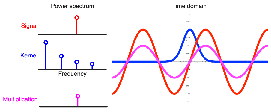
This provides a different perspective on convolutions by thinking of convolutions as spectral filters. Consider a sine wave with a frequency at \(f\) convolved with a gaussian kernel. The power spectra of a pure sine wave has a bar at the frequency \(f\). The power spectra of a gaussian kernel is a negative exponential. The narrower the gaussian we get a more gentle exponential decay in the frequency domain. If we multiply the two power spectra element-wise, we get basically zeros everywhere the two power spectra do not overlap. Only at the frequency \(f\) we get a non-zero value. Convolution in the time domain is equivalent to multiplication in the frequency domain.

I think this is a very intuitive way to understand why convolutions work. A convolution filters out the frequencies that are not present in both the signal and the kernel. Only the features of the signal that share characteristics with the features in the kernel are amplitude modulated and preserved in the output.

We can do some other interesting things in the frequency domain, like filtering out noise and reconstructing the signal using the inverse Fourier transform. Let’s see how we can decompose a signal into its frequency components using the FFT and reconstruct the signal using the iFFT.

Given a time series of values value and timesteps ts, the rFFT of the signal is computed using the following code snippet. We first detrend the signal by subtracting the mean and dividing by the standard deviation (z-score). This removes the zero-Hz fequency (DC offset), which would otherwise dominate the power spectrum. We then compute the rFFT of the detrended signal to get the complex values (amplitude and phase). The amplitudes are the absolute values of the complex values. The frequencies are computed using the rfftfreq function.

# Examine the PSD using the rFFT
xmean = np.mean(value)
xvar = np.var(value)
zvalues = (value - xmean) / np.sqrt(xvar)
tsnorm = (ts - ts[0]) / (ts[-1] - ts[0])
rfft_values = np.fft.rfft(zvalues)  # complex values
amplitudes = np.abs(rfft_values)  # amplitudes
freqs = np.fft.rfftfreq(len(value), d=tsnorm[1] - tsnorm[0])

We plot the power spectral density (PSD) of the signal, which tells us the energy at each frequency.

Since period is the inverse of frequency, by identifying the frequencies that carry most of the energy, we can also discover the most dominant periods. The signal has a few dominant frequencies. We can select the top-5 frequencies (10.96, 9.96, 20.92, 21.91, 4.98) and reconstruct the signal using the inverse Fourier transform. This is equivalent to filtering for frequencies that capture most of the signal energy and removing the rest. This allows us to denoise the signal by removing the high-frequency components. Notice the reconstructed signal is a smoothed version of the original signal.

# Extract the top 5 dominant frequencies
top5 = np.argsort(amplitudes)[::-1][:5]
top5_freqs = freqs[top5]
print("Top 5 frequencies:", top5_freqs.round(2))

# Reconstruct the signal using the top 5 frequencies
rfft_values_filtered = np.zeros_like(rfft_values)
rfft_values_filtered[top5] = rfft_values[top5]
recon = np.fft.irfft(rfft_values_filtered)
recon = recon * np.sqrt(xvar) + xmean

You can also low-pass filter the signal by setting an upper-bound on the cut-off frequency and setting all amplitudes above the cut-off frequency to zero, then reconstruct the signal using the inverse Fourier transform.

Finally, we can implement a 1D convolution using the FFT in PyTorch.

import torch
import torch.fft as fft
from scipy.fftpack import next_fast_len

def conv1d_fft(signal: torch.Tensor, kernel: torch.Tensor, dim: int=-1):
    """Convolve two 1D tensors using FFT.

    Args:
        signal (Tensor): Shape (batch_size, N) where N is the signal length
        kernel (Tensor): Shape (batch_size, M) where M is the kernel length
        dim (int, optional): Dimension along which to convolve. Default is -1.

    Returns:
        Tensor: Shape (batch_size, N) containing the convolved signal
    """
    N = signal.size(dim)  # signal length
    M = kernel.size(dim)  # kernel length

    fast_len = next_fast_len(N + M - 1)

    F_f = fft.rfft(signal, fast_len, dim=dim)  # shape (N, fast_len // 2 + 1)
    F_g = fft.rfft(kernel, fast_len, dim=dim)  # shape (N, fast_len // 2 + 1)

    F_fg = F_f * F_g.conj()
    out = fft.irfft(F_fg, fast_len, dim=dim)
    out = out.roll((-1,), dims=(dim,))
    idx = torch.as_tensor(range(fast_len - N, fast_len)).to(out.device)
    out = out.index_select(dim, idx)

    return out